# Uncomment and run if using Colab!

#import urllib.request
#remote_url = 'https://gist.githubusercontent.com/gabehope/d3e6b10338a1ba78f53204fc7502eda5/raw/52631870b1475b5ef8d9701f1c676fa97bf7b300/hw5_support.py'
#with urllib.request.urlopen(remote_url) as remote, open('hw6_support.py', 'w') as local:
#  [local.write(str(line, encoding='utf-8')) for line in remote]

# Run me first!
from hw6_support import *Homework 6: Vectorization (solutions)
Overview
In this homework we will update a our reverse-mode automatic differentiation library to use vectorized operations. It should make it a lot faster!
Python features
This homework makes use of a few fancy features in Python that are worth knowing about if you are unfamiliar. - Variable length arguments (e.g. *args) - List comprehensions (e.g. [a**2 for a in range(5)]) - Magic methods (e.g. __add__)
Part 0: Setting up automatic differentiation
Here we’ll re-use our automatic differentiation library from the previous homework as our starting point for this assignment.
In the marked cells below, copy the corresponding answers from homework 5. You may use either your own answers or published solutions.
class AutogradValue:
    '''
    Base class for automatic differentiation operations. Represents variable delcaration.
    Subclasses will overwrite func and grads to define new operations.

    Properties:
        parents (list): A list of the inputs to the operation, may be AutogradValue or float
        parent_values    (list): A list of raw values of each input (as floats)
        forward_grads (dict): A dictionary mapping inputs to gradients
        grad    (float): The derivative of the final loss with respect to this value (dL/da)
        value   (float): The value of the result of this operation
    '''

    def __init__(self, *args):
        self.parents = list(args)
        self.parent_values = [arg.value if isinstance(arg, AutogradValue) else arg for arg in args]
        self.forward_grads = {}
        self.value = self.forward_pass()
        self.grad = 0. # Used later for reverse mode

    def func(self, input):
        '''
        Compute the value of the operation given the inputs.
        For declaring a variable, this is just the identity function (return the input).

        Args:
            input (float): The input to the operation
        Returns:
            value (float): The result of the operation
        '''
        return input

    def grads(self, *args):
        '''
        Compute the derivative of the operation with respect to each input.
        In the base case the derivative of the identity function is just 1. (da/da = 1).

        Args:
            input (float): The input to the operation
        Returns:
            grads (tuple): The derivative of the operation with respect to each input
                            Here there is only a single input, so we return a length-1 tuple.
        '''
        return (1,)

    def forward_pass(self):
        # Calls func to compute the value of this operation
        return self.func(*self.parent_values)

    def __repr__(self):
        # Python magic function for string representation.
        return str(self.value)
Defining operations
Copy the corresponding answers from homework 5 here. You may use either your own answers or published solutions.
class _add(AutogradValue):
    def func(self, a, b):
        return a + b

    def grads(self, a, b):
        return 1., 1.

class _sub(AutogradValue):
    def func(self, a, b):
        return a - b

    def grads(self, a, b):
        return 1., -1.

class _neg(AutogradValue):
    def func(self, a):
        return -a

    def grads(self, a):
        return (-1.,)

class _mul(AutogradValue):
    def func(self, a, b):
        return a * b

    def grads(self, a, b):
        return b, a

class _div(AutogradValue):
    def func(self, a, b):
        return a / b

    def grads(self, a, b):
        return 1 / b, -a / (b * b)

class _exp(AutogradValue):
    def func(self, a):
        return math.exp(a)

    def grads(self, a):
        return (math.exp(a),)

class _log(AutogradValue):
    def func(self, a):
        return math.log(a)

    def grads(self, a):
        return (1 / a,)
Backward pass
Copy the corresponding answers from homework 5 here. You may use either your own answers or published solutions.
def backward_pass(self):
    local_grads = self.grads(*self.parent_values)

    # Loop through pairs of parents and their corresponding grads
    for node, grad in zip(self.parents, local_grads):
        # Update the gradient of each AutogradValue parent
        if isinstance(node, AutogradValue):
            node.grad += self.grad * grad

AutogradValue.backward_pass = backward_pass
def backward(self):
# We call backward on the loss, so dL/dL = 1
self.grad = 1.
queue = [self]
order = []
# Additionally keep track of the visit counts for each node
counts = {}
while len(queue) > 0:
node = queue.pop()
# Rather than removing nodes from the order [slow, O(N)],
# just mark that it has been visited again [O(1)]
if isinstance(node, AutogradValue):
if node in counts:
counts[node] += 1
else:
counts[node] = 1
order.append(node)
queue.extend(node.parents)
# Go through the order, but only call backward pass once we're at
# the last vist for a given node
for node in order:
counts[node] -= 1
if counts[node] == 0:
node.backward_pass()
AutogradValue.backward = backwarddef exp(a):
return _exp(a) if isinstance(a, AutogradValue) else math.exp(a)
def log(a):
return _log(a) if isinstance(a, AutogradValue) else math.log(a)
# Note: Remember that above we defined a class for each type of operation
# so in this code we are overriding the basic operators for AutogradValue
# such that they construct a new object of the class corresponding to the
# given operation and return it.
# (You don't need to everything that's happening here to do the HW)
AutogradValue.exp = lambda a: _exp(a)
AutogradValue.log = lambda a: _log(a)
AutogradValue.__add__ = lambda a, b: _add(a, b)
AutogradValue.__radd__ = lambda a, b: _add(b, a)
AutogradValue.__sub__ = lambda a, b: _sub(a, b)
AutogradValue.__rsub__ = lambda a, b: _sub(b, a)
AutogradValue.__neg__ = lambda a: _neg(a)
AutogradValue.__mul__ = lambda a, b: _mul(a, b)
AutogradValue.__rmul__ = lambda a, b: _mul(b, a)
AutogradValue.__truediv__ = lambda a, b: _div(a, b)
AutogradValue.__rtruediv__ = lambda a, b: _div(b, a)Training a neural network
Now we’re ready to test out our AutogradValue implementation in the context it’s designed for: neural networks!
def pad(a):
    # Pads an array with a column of 1s (for bias term)
    return a.pad() if isinstance(a, AutogradValue) else np.pad(a, ((0, 0), (0, 1)), constant_values=1., mode='constant')

def matmul(a, b):
    # Multiplys two matrices
    return _matmul(a, b) if isinstance(a, AutogradValue) or isinstance(b, AutogradValue) else np.matmul(a, b)

def sigmoid(x):
    # Computes the sigmoid function
    return 1. / (1. + (-x).exp()) if isinstance(x, AutogradValue) else 1. / (1. + np.exp(-x))

def log(x):
    # Computes the sigmoid function
    return x.log() if isinstance(x, AutogradValue) else np.log(x)

class NeuralNetwork:
    def __init__(self, dims, hidden_sizes=[]):
        # Create a list of all layer dimensions (including input and output)
        sizes = [dims] + hidden_sizes + [1]
        # Create each layer weight matrix (including bias dimension)
        self.weights = [np.random.normal(scale=1., size=(i + 1, o))
                        for (i, o) in zip(sizes[:-1], sizes[1:])]

    def prediction_function(self, X, w):
        '''
        Get the result of our base function for prediction (i.e. x^t w)

        Args:
            X (array): An N x d matrix of observations.
            w (list of arrays): A list of weight matrices
        Returns:
            pred (array): An N x 1 matrix of f(X).
        '''
        # Iterate through the weights of each layer and apply the linear function and activation
        for wi in w[:-1]:
            X = pad(X) # Only if we're using bias
            X = sigmoid(matmul(X, wi))

        # For the output layer, we don't apply the activation
        X = pad(X)
        return matmul(X, w[-1])

    def predict(self, X):
        '''
        Predict labels given a set of inputs.

        Args:
            X (array): An N x d matrix of observations.
        Returns:
            pred (array): An N x 1 column vector of predictions in {0, 1}
        '''
        return (self.prediction_function(X, self.weights) > 0)

    def predict_probability(self, X):
        '''
        Predict the probability of each class given a set of inputs

        Args:
            X (array): An N x d matrix of observations.
        Returns:
            probs (array): An N x 1 column vector of predicted class probabilities
        '''
        return sigmoid(self.prediction_function(X, self.weights))

    def accuracy(self, X, y):
        '''
        Compute the accuracy of the model's predictions on a dataset

        Args:
            X (array): An N x d matrix of observations.
            y (array): A length N vector of labels.
        Returns:
            acc (float): The accuracy of the classifier
        '''
        y = y.reshape((-1, 1))
        return (self.predict(X) == y).mean()

    def nll(self, X, y, w=None):
        '''
        Compute the negative log-likelihood loss.

        Args:
            X (array): An N x d matrix of observations.
            y (array): A length N vector of labels.
            w (array, optional): A (d+1) x 1 matrix of weights.
        Returns:
            nll (float): The NLL loss
        '''
        if w is None:
            w = self.weights

        y = y.reshape((-1, 1))
        xw = self.prediction_function(X, w)
        py = sigmoid(xw * (2 * y - 1))
        nll = -(log(py))
        return nll.sum()
Autograd for a neural network
Copy the corresponding answers from homework 5 here. You may use either your own answers or published solutions.
def element_map(f, a):
    '''
    Creates a new array the same shape as a, with a function f applied to each element.

    Args:
        a (function): The function to apply
        a (array): The array to map
    Returns:
        g (array): An array g, such that g[i,j] = f(a[i,j])
    '''

    # Store the original shape
    shape = a.shape

    # Create a 1-d array with the same elements using flatten()
    # then iterate through applying f to each element
    flat_wrapped = np.asarray([f(ai) for ai in a.flatten()])

    # Reshape back to the original shape
    return flat_wrapped.reshape(shape)

def wrap_array(a):
    '''
    Wraps the elements of an array with AutogradValue

    Args:
        a (array of float): The array to wrap
    Returns:
        g (array of AutogradValue): An array g, such that g[i,j] = AutogradValue(a[i,j])
    '''
    return element_map(AutogradValue, a)


def unwrap_gradient(a):
    '''
    Unwraps the gradient of an array with AutogradValues

    Args:
        a (array of AutogradValue): The array to unwrap
    Returns:
        g (array of float): An array g, such that g[i,j] = a[i,j].grad
    '''
    return element_map(lambda ai: ai.grad, a)
def nll_and_grad(self, X, y):
'''
Get the negative log-likelihood loss and its gradient
Args:
X (array): An N x d matrix of observations.
y (array): A length N vector of labels
Returns:
nll (float): The negative log-likelihood
grads (list of arrays): A list of the gradient of the nll with respect
to each value in self.weights.
'''
# Wrap the array we want to differentiate with respect to (weights)
w = [wrap_array(wi) for wi in self.weights]
# Run the NLL function and call backward to populate the gradients
nll = self.nll(X, y, w)
nll.backward()
# Get both the nll value and graident
return nll.value, [unwrap_gradient(wi) for wi in w]
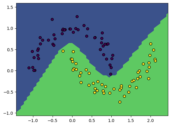
NeuralNetwork.nll_and_grad = nll_and_gradWe now have everything in place to train a neural network from scratch! Let’s try it on our tiny dataset. Feel free to change the inputs.
X, y = make_moons(100, noise=0.1)
model = NeuralNetwork(2, [5, 5])
gradient_descent(model, X, y, lr=3e-2, steps=250)

print('Model accuracy: %.3f' % model.accuracy(X, y))
plot_boundary(model, X, y)
Loss 3.60, accuracy: 0.99: 100%|██████████| 250/250 [00:12<00:00, 20.36it/s] Model accuracy: 0.990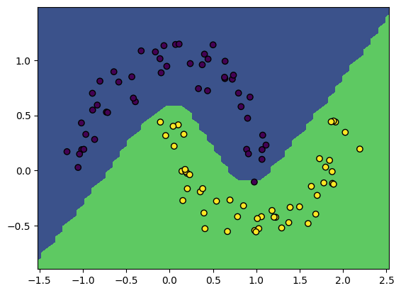
Part 1: Vectorizing Reverse-mode automatic differentiation
We might notice that our reverse-mode automatic differentiation implementation is quite slow! The main reason for this is that our implementation operates on individual numbers (scalars) rather than entire arrays. This means that for a big operation like a matrix multiplication, an AutogradValue object needs to be tracked for each of the \(O(n^3)\) individual operations! Even worse, it also means that internally Numpy can’t use the very fast C and C++ implementations it has for array operations on type float, our array elements are now objects so it has to fall back on slow Python-loop based implementations.
Ideally we’d like our AutogradValue objects to operate at the level of array operations, rather than scalar operations. This would circumvent these problems as we could represent an entire matrix multiplication with a single AutogradValue. In order to do this efficiently, we’ll need to make use of the Vector-Jacobian Product idea that we discussed in class. Let’s review the concept here.
Recall that in backward_pass for a node c we assume that we have the gradient (derivative) of the loss with respect to c: \(\frac{dL}{d\mathbf{c}}\) and we need to update the gradients for the parents (say a and b) as:
\[\frac{dL}{da} = \frac{dL}{dc} \frac{dc}{da}, \quad \frac{dL}{dc} = \frac{dL}{dc} \frac{dc}{db}\]
When \(\mathbf{a}\), \(\mathbf{b}\) and \(\mathbf{c}\) are vectors the derivates \(\frac{d\mathbf{c}}{d\mathbf{a}}\) and \(\frac{d\mathbf{c}}{d\mathbf{b}}\) are Jacobian matrices with possibly many entries and our updates become vector-Jacobian products:
\[\frac{dL}{d\mathbf{a}} = \bigg(\frac{dL}{d\mathbf{c}}^T \frac{d\mathbf{c}}{d\mathbf{a}}\bigg)^T, \quad \frac{dL}{d\mathbf{b}} = \bigg(\frac{dL}{d\mathbf{c}}^T \frac{d\mathbf{c}}{d\mathbf{b}}\bigg)^T\]
Q1
In this case, let’s assume that \(\mathbf{a}\) is a length \(n\) vector and \(\mathbf{c}\) is a length \(m\) vector. So we would say that: \[\mathbf{a} \in \mathbb{R}^n, \quad \mathbf{c} \in \mathbb{R}^m\]
Remember that our loss, \(L\), is generally a scalar (\(L\in \mathbb{R}\)). Based on this, what is the shape of each term in the equation below?
\[\frac{dL}{d\mathbf{a}} = \bigg(\frac{dL}{d\mathbf{c}}^T \frac{d\mathbf{c}}{d\mathbf{a}}\bigg)^T\]
Your answer should be as matrix/vector dimensions e.g. \((n \times m)\)
Answer
\[\frac{dL}{d\mathbf{a}} = (n)\] \[\frac{dL}{d\mathbf{c}} = (m)\] \[\frac{d\mathbf{c}}{d\mathbf{a}} = (m \times n)\]
Element-wise operations
We often don’t need to actually construct the Jacobians fully to compute these vector-Jacobian products, as is the case for element-wise operations. As long as we can compute the correct values for \(\frac{dL}{d\mathbf{a}}\), we’re good! For example if \[\mathbf{c} = \mathbf{a}^2, \quad \mathbf{c} = \begin{bmatrix} a_1^2 \\ a_2^2 \\ a_3^2 \\ \vdots \end{bmatrix}\]
We can easily see that we can just update the derivate for each element of \(\mathbf{a}\) independently. \[\frac{dL}{d\mathbf{a}} = \begin{bmatrix} \frac{dL}{dc_1} \cdot 2 a_1 \\ \frac{dL}{dc_2} \cdot 2 a_2 \\ \frac{dL}{dc_3} \cdot 2 a_3 \\ \vdots \end{bmatrix} = 2 \mathbf{a} \odot \frac{dL}{d\mathbf{c}}\]
If we want to be more formal we can note that technically, the Jacobian \(\frac{d\mathbf{c}}{d\mathbf{a}}\) is diagonal (\(\frac{\partial c_i}{\partial a_j}\) is only nonzeros for \(i=j\)). Therefore we can write the Vector-Jacobian Product as:
\[\frac{dL}{d\mathbf{a}}^T = \frac{dL}{d\mathbf{c}}^T \frac{d\mathbf{c}}{d\mathbf{a}} = \begin{bmatrix} \frac{dL}{dc_1} \\ \frac{dL}{dc_2} \\ \frac{dL}{dc_3} \\ \vdots \end{bmatrix}^T \begin{bmatrix} 2 a_1 & 0 & 0 & \dots \\0 & 2 a_2 & 0 & \dots \\ 0 & 0 & 2 a_3 & \dots \\ \vdots & \vdots & \vdots & \ddots \end{bmatrix} = \begin{bmatrix} \frac{dL}{dc_1} \cdot 2 a_1 \\ \frac{dL}{dc_2} \cdot 2 a_2 \\ \frac{dL}{dc_3} \cdot 2 a_3 \\ \vdots \end{bmatrix}^T = \bigg(2 \mathbf{a} \odot \frac{dL}{d\mathbf{c}}\bigg)^T\]
For the case of addition, things are even simpler! If: \[\mathbf{c} = \mathbf{a} + \mathbf{b}\]
We can again see that we can just update the derivative for each element of \(\mathbf{a}\) independently, but this time each local derivative (\(\frac{dc_i}{da_i}\)) is just \(1\), so \[\frac{dL}{d\mathbf{a}} = \begin{bmatrix} \frac{dL}{dc_1} \cdot 1 \\ \frac{dL}{dc_2} \cdot 1 \\ \frac{dL}{dc_3} \cdot 1 \\ \vdots \end{bmatrix} = \frac{dL}{d\mathbf{c}}\]
In this case the Jacobian \(\frac{d\mathbf{c}}{d\mathbf{a}}\) is simply the identity matrix, so: \[\frac{dL}{d\mathbf{a}}^T = \begin{bmatrix} \frac{dL}{dc_1} \\ \frac{dL}{dc_2} \\ \frac{dL}{dc_3} \\ \vdots \end{bmatrix}^T \begin{bmatrix} 1 & 0 & 0 & \dots \\0 & 1 & 0 & \dots \\ 0 & 0 & 1 & \dots \\ \vdots & \vdots & \vdots & \ddots \end{bmatrix}= \frac{dL}{d\mathbf{c}}^T \mathbf{I} = \frac{dL}{d\mathbf{c}}^T\]
Q2
Assume that we have the following formula for \(\mathbf{a}\): \[\mathbf{a}= \exp \big( \mathbf{A} \mathbf{w} \big) + \mathbf{w}^2\] Where \(\mathbf{A}\) is a constant \(n \times n\) matrix. Given the gradient of \(L\) with respect to \(\mathbf{a}\): \(\frac{dL}{d\mathbf{a}}\), what is the gradient of \(L\) with respect to \(\mathbf{w}\) (\(\frac{dL}{d\mathbf{w}}\)) in terms of: \(\frac{dL}{d\mathbf{a}}\), \(\mathbf{A}\) and \(\mathbf{w}\)?
Hint: You do not need to write a formula for the Jacobian (\(\frac{d\mathbf{a}}{d\mathbf{w}}\)). As we see above, many VJPs can be written without definining the Jacobian explicitly (e.g. for element-wise functions). You can use \(\odot\) (\odot) to denote an element-wise product between vectors: \[ \mathbf{a} \odot \mathbf{b} = \begin{bmatrix}
a_1 b_1 \\
a_2 b_3 \\
\vdots \\
a_d b_d \\
\end{bmatrix}
\]
Answer
Here we’ll start by writing out the vector-Jacobian product we’re looking for: \[\frac{dL}{d\mathbf{w}} = \frac{dL}{d\mathbf{a}}^T\frac{d\mathbf{a}}{d\mathbf{w}} = \frac{dL}{d\mathbf{a}}^T\frac{d}{d\mathbf{w}}\bigg( \exp \big( \mathbf{A} \mathbf{w} \big) + \mathbf{w}^2\bigg)\] Using the addition rule, we can distribute the derivative: \[=\frac{dL}{d\mathbf{a}}^T\frac{d}{d\mathbf{w}}\bigg( \exp \big( \mathbf{A} \mathbf{w} \big)\bigg) + \frac{dL}{d\mathbf{a}}^T\frac{d}{d\mathbf{w}}\bigg(\mathbf{w}^2\bigg)\]
For simplicity, let’s substitute \(\mathbf{b} = \mathbf{A}\mathbf{w}\) for now, so we can apply the chain rule \[=\frac{dL}{d\mathbf{a}}^T\frac{d}{d\mathbf{b}}\bigg( \exp \big( \mathbf{b} \big)\bigg)\frac{d\mathbf{b}}{d\mathbf{w}} + \frac{dL}{d\mathbf{a}}^T\frac{d}{d\mathbf{w}}\bigg(\mathbf{w}^2\bigg)\]
We see that \(\exp(w)\) and \(w^2\) are both element-wise operations, so we can use the rule we learned in class:
\[ = \bigg(\frac{dL}{d\mathbf{a}} \odot \exp(d\mathbf{b})\bigg)^T \frac{d\mathbf{b}}{d\mathbf{w}} + 2 \bigg( \frac{dL}{d\mathbf{a}} \odot \mathbf{w} \bigg)\]
Finally we know that \(\mathbf{b} = \mathbf{A}\mathbf{w}\), therefore \(\frac{d\mathbf{b}}{d\mathbf{w}} = \mathbf{A}\)
\[ \frac{dL}{d\mathbf{w}} = \bigg(\frac{dL}{d\mathbf{a}} \odot \exp(\mathbf{A}\mathbf{w})\bigg)^T \mathbf{A} + 2 \bigg( \frac{dL}{d\mathbf{a}} \odot \mathbf{w} \bigg)\]
Q3
Let’s replace our operation implementations above with ones that compute Vector-Jacobian products. We’ll start with element-wise operations. Complete the vjp function for each operation below. Unlike the grads methods we implemented before which computed the derivative of the output with respect to each input: \(\frac{dc}{da}\) and \(\frac{dc}{db}\) (if applicable), each vjp method should directly compute the gradient of the loss with respect to each input: \(\frac{dL}{d\mathbf{a}}\) and \(\frac{dL}{d\mathbf{b}}\), assuming the grad argument provides the gradient of the loss with respect to the output: \(\frac{dL}{d\mathbf{c}}\).
Hint: For binary operations (+,-,*,/), you do not need to account for broadcasting. That is, you can assume that a, b and c are always the same shape! We’ve started you off with a few examples to base your answers on.
class _add(AutogradValue):
    # An example representing the addition operation.
    def func(self, a, b):
        '''
        Computes the result of the operation (a + b). Assumes a and b are the same shape.

        Args:
            a (array of float): The first operand
            b (array of float): The second operand
        Returns:
            c (array of float): The result c = a + b
        '''
        return a + b

    def vjp(self, grad, a, b):
        '''
        Computes dL/da and dL/db given dL/dc.

        Args:
            grad (array of float): The gradient of the loss with respect to the output (dL/dc)
            a (array of float): The first operand
            b (array of float): The second operand
        Returns:
            grads (tuple of arrays): A tuple containing the gradients dL/da and dL/db
        '''
        return grad, grad

class _square(AutogradValue):
    # Another example class implementing c = a^2
    def func(self, a):
        return a ** 2

    def vjp(self, grad, a):
        return (2 * a * grad,)

class _pad(AutogradValue):
    # An implementation for padding with a column of 1s.
    def func(self, a):
        return np.pad(a, ((0, 0), (0, 1)), constant_values=1., mode='constant')

    def vjp(self, grad, a):
        return (grad[:, :-1],)
Answer
class _sub(AutogradValue):
    def func(self, a, b):
        return a - b

    def vjp(self, grad, a, b):
        return grad, -grad

class _neg(AutogradValue):
    def func(self, a):
        return -a

    def vjp(self, grad, a):
        return (-grad,)

class _mul(AutogradValue):
    def func(self, a, b):
        return a * b

    def vjp(self, grad, a, b):
        return b * grad, a * grad

class _div(AutogradValue):
    def func(self, a, b):
        return a / b

    def vjp(self, grad, a, b):
        return grad / b, grad * (-a / (b * b))

class _exp(AutogradValue):
    def func(self, a):
        return np.exp(a)

    def vjp(self,grad,  a):
        return (grad * np.exp(a),)

class _log(AutogradValue):
    def func(self, a):
        return np.log(a)

    def vjp(self, grad, a):
        return (grad / a,)

test_vjp(_neg, '_neg', )
test_vjp(_exp, '_exp', true_func=anp.exp)
test_vjp(_log, '_log', true_func=anp.log)
test_vjp(_sub, '_sub', True)
test_vjp(_mul, '_mul', True)
test_vjp(_div, '_div', True)
Passed _neg!
Passed _exp!
Passed _log!
Passed _sub!
Passed _mul!
Passed _div!Q4
Consider the operation defined by np.sum, that takes the sum over all elements of a matrix or vector, producing a scalar:
\[c = \sum_{i=1}^n a_i\]
Write a vjp method for this operation that computes: \(\frac{dL}{d\mathbf{a}}\) given \(\frac{dL}{dc}\).
Hint: Note that \(L\), \(c\) and \(\frac{dL}{dc}\) are all scalars, so for any entry \(i\) of our output we can simply apply the chain rule and compute \(\frac{dL}{da_i} = \frac{dL}{dc} \frac{dc}{da_i}\). As the equation above for \(c\) given \(\mathbf{a}\) is a sum, \(\frac{dc}{da_i}\) should be simple!
Answer
class _sum(AutogradValue):
    def func(self, a):
        return np.sum(a)

    def vjp(self, grad, a):
        return (grad * np.ones_like(a),)

test_vjp(_sum, '_sum', true_func=anp.sum, issum=True)
Passed _sum!Matrix multiplication
For the next few problems, it may be useful to refer to this diagram of matrix multiplication.

The last important operation we’ll need a vjp method for in order to use our vectorized AutogradValue class for a neural network is matrix multiplication. Let’s consider the operation:
\[\mathbf{C} = \mathbf{A}\mathbf{B}\]
Where \(\mathbf{A}\) is an \(N\times h\) matrix, \(\mathbf{B}\) is a \(h \times d\) matrix and \(\mathbf{C}\) is an \(N\times d\) matrix.
Recall that for vjp want to compute \(\frac{dL}{d\mathbf{A}}\) (and \(\frac{dL}{d\mathbf{B}}\) ) given \(\frac{dL}{d\mathbf{C}}\). We can compute a given entry \(i,j\) of \(\frac{dL}{d\mathbf{A}}\) by applying the chain rule using each element of \(\mathbf{C}\):
\[\frac{dL}{dA_{ij}} = \sum_{k=1}^N \sum_{l=1}^d \frac{dL}{dC_{kl}}\frac{dC_{kl}}{dA_{ij}}\]
However, each entry of \(\mathbf{C}\) only depends on a single row of \(\mathbf{A}\) and a single column of \(\mathbf{B}\), thus for most \(i,j,k,l\), \(\frac{dC_{kl}}{dA_{ij}}=0\).
Q5
Using this observation, simplify the expression for \(\frac{dL}{dA_{ij}}\) above. (The derivative of the loss with respect to the entry of \(\mathbf{A}\) at row \(i\), column \(j\)).
Hint: Your answer should have a similar form, but should only have a single summation and a subset of the indices \(i,j,k,l\).
Answer
\[\frac{dL}{dA_{ij}} = \sum_{l=1}^d \frac{dL}{dC_{il}}\frac{dC_{il}}{dA_{ij}}\]
Q6
Recalling the definition of matrix-multiplication, give a simple expression for \(\frac{dC_{il}}{dA_{ij}}\), then substitue it into your expression for \(\frac{dL}{dA_{ij}}\).
Answer
\[\frac{dC_{il}}{dA_{ij}}=B_{jl} , \quad\frac{dL}{dA_{ij}} = \frac{dL}{dC_{il}}B_{jl}\]
Q7
Using your expression in Q13, write an expression for \(\frac{dL}{d\mathbf{A}}\) as a matrix multiplication between two of the 3 given matrices: \(\frac{dL}{d\mathbf{C}}\), \(\mathbf{A}\), \(\mathbf{B}\). Make sure to inlude any nessecary transposes.
Hint: Recall that \(\frac{dL}{d\mathbf{C}}\) is the same shape as \(\mathbf{C}\) (\(N\times d\)), \(\mathbf{A}\) has shape \(N \times h\) and \(\mathbf{B}\) has shape \(h \times d\).
Answer
\[\frac{dL}{d\mathbf{A}}= \frac{dL}{d\mathbf{C}}\mathbf{B}^T\]
Q8
Write the corresponding formula for \(\frac{dL}{d\mathbf{B}}\).
Hint: You can use the fact that \(C^T = B^T A^T\) and that \(\frac{dL}{d\mathbf{C}^T} = (\frac{dL}{d\mathbf{C}})^T\)
Answer
\[\frac{dL}{d\mathbf{B}}=\frac{dL}{d\mathbf{C}}^T\mathbf{A}\]
Q9
Using the expressions you derived in Q14 and Q15, implement the vjp function for the matmul operation to compute \(\frac{dL}{d\mathbf{A}}\) and \(\frac{dL}{d\mathbf{B}}\) given \(\frac{dL}{d\mathbf{C}}\), \(\mathbf{A}\) and \(\mathbf{B}\).
Answer
class _matmul(AutogradValue):
    def func(self, a, b):
        return np.matmul(a, b)

    def vjp(self, grad, a, b):
        return np.dot(grad, b.T), np.dot(grad.T, a).T

test_vjp(_matmul, '_matmul', binary=True, true_func=anp.matmul)
Passed _matmul!Now that we’ve written the vjp versions of our operators, we’ll update our AutogradValue class to use them!
# Note: Remember that above we defined a class for each type of operation
# so in this code we are overriding the basic operators for AutogradValue
# such that they construct a new object of the class corresponding to the
# given operation and return it.
# (You don't need to everything that's happening here to do the HW)
AutogradValue.vjp = lambda self, g, a: (1.,)
AutogradValue.exp = lambda a: _exp(a)
AutogradValue.log = lambda a: _log(a)
AutogradValue.pad = lambda a: _pad(a)
AutogradValue.sum = lambda a: _sum(a)
AutogradValue.matmul = lambda a, b: _matmul(a, b)
AutogradValue.__add__ = lambda a, b: _add(a, b)
AutogradValue.__radd__ = lambda a, b: _add(b, a)
AutogradValue.__sub__ = lambda a, b: _sub(a, b)
AutogradValue.__rsub__ = lambda a, b: _sub(b, a)
AutogradValue.__neg__ = lambda a: _neg(a)
AutogradValue.__mul__ = lambda a, b: _mul(a, b)
AutogradValue.__rmul__ = lambda a, b: _mul(b, a)
AutogradValue.__truediv__ = lambda a, b: _div(a, b)
AutogradValue.__rtruediv__ = lambda a, b: _div(b, a)
As a final step, we need to update our backward_pass method to use our new vjp method instead of relying on grads.
Q10
Update your backward_pass method to use vjp instead of grads.
Hint: Recall that vjp directly computes \(\frac{dL}{d\mathbf{a}}\), \(\frac{dL}{d\mathbf{b}}\), whereas grads computed \(\frac{dc}{da}\), \(\frac{dc}{db}\)
Answer
def backward_pass(self):
    local_vjps = self.vjp(self.grad, *self.parent_values)
    # Loop through pairs of parents and their corresponding grads
    for node, vjp in zip(self.parents, local_vjps):
        # Update the gradient of each AutogradValue parent
        if isinstance(node, AutogradValue):
            node.grad += vjp

AutogradValue.backward_pass = backward_pass
Q11
Finally update the nll_and_grad function for our NeuralNetwork class to use our shiny new vectorized reverse-mode implementation.
Hint: We should no longer need to use our wrap_array and unwrap_gradient functions, as AutogradValue objects can now contain arrays!
Answer
def nll_and_grad(self, X, y):
    '''
    Get the negative log-likelihood loss and its gradient

    Args:
        X (array): An N x d matrix of observations.
        y (array): A length N vector of labels
    Returns:
        nll (float): The negative log-likelihood
        grads (list of arrays): A list of the gradient of the nll with respect
                                to each value in self.weights.
    '''
    w = [AutogradValue(wi) for wi in self.weights]
    nll = self.nll(X, y, w)
    nll.backward()
    return nll.value, [wi.grad for wi in w]

NeuralNetwork.nll_and_grad = nll_and_grad
We should be able to run it with a much larger network now!
X, y = make_moons(100, noise=0.1)
model = NeuralNetwork(2, [25, 25])
gradient_descent(model, X, y, lr=3e-2, steps=250)

print('Model accuracy: %.3f' % model.accuracy(X, y))
plot_boundary(model, X, y)
Loss 2.37, accuracy: 1.00: 100%|██████████| 250/250 [00:00<00:00, 1332.97it/s]Model accuracy: 1.000